-
Summarize a complete book using the giant context window in Gemini 1.5
A short (< 10-minute) demo video, with a couple of intro comments about early 2024 LLM developments
-
Generative AI in 2024
A slide presentation for a discussion with HBS Next Chapter.
-
Practical ChatGPT Prompting: 15 Patterns to Improve Your Prompts
A logician is hiking through snowy woods and sees a small spaceship, and next to it, two tiny legs, sticking out of a snow drift. He digs the little creature out, and it turns out to be small omniscient space alien. The alien is extremely grateful and, being omniscient, offers to answer any question the logician may have. Naturally the logician asks: “What is the best question to ask and what is the correct answer to that question?” The tiny alien pauses momentarily, and replies, “The best question is the one you just asked; and the correct answer is this one.” And just like that…the alien hops in their spaceship and flies away.

Image via Dall-E: An image in the style of an arty Japanese animated film with vibrant colors, side view of a young lady sitting at a desk in front of a laptop in a library, looking dreamy and inquisitive. On her laptop screen, a futuristic robot is depicted sitting at a sleek desk facing the young lady. -
OpenAI DevDay
OpenAI is moving fast and extending their lead.
-
Truth, Lies, and ChatGPT
There are three kinds of lies: lies, damned lies, and statistics. - Mark Twain
-
Bullshit
That was just bullshit, Joel. - Miles, in Risky Business (1983)
History is a set of lies agreed upon. - Napoleon Bonaparte
Bullshit is the glue that binds us as a nation. - George Carlin

-
ChatGPT, OpenAI, and the Generative AI Revolution
I think it’s comparable in scale with the Industrial Revolution or electricity — or maybe the wheel. - Geoffrey Hinton
Any sufficiently advanced technology is indistinguishable from magic. - Arthur C. Clarke
GPT is a transformer so smart / That can write like a human or a bard / It can answer your queries / Or make stories so eerie / That you’ll wonder if it has a heart - GPT
-
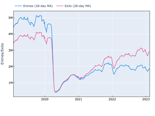
NYC Subways and the Terrible, Horrible, No Good, Very Bad, Turnstile Data
The future ain’t what it used to be. - Yogi Berra
-
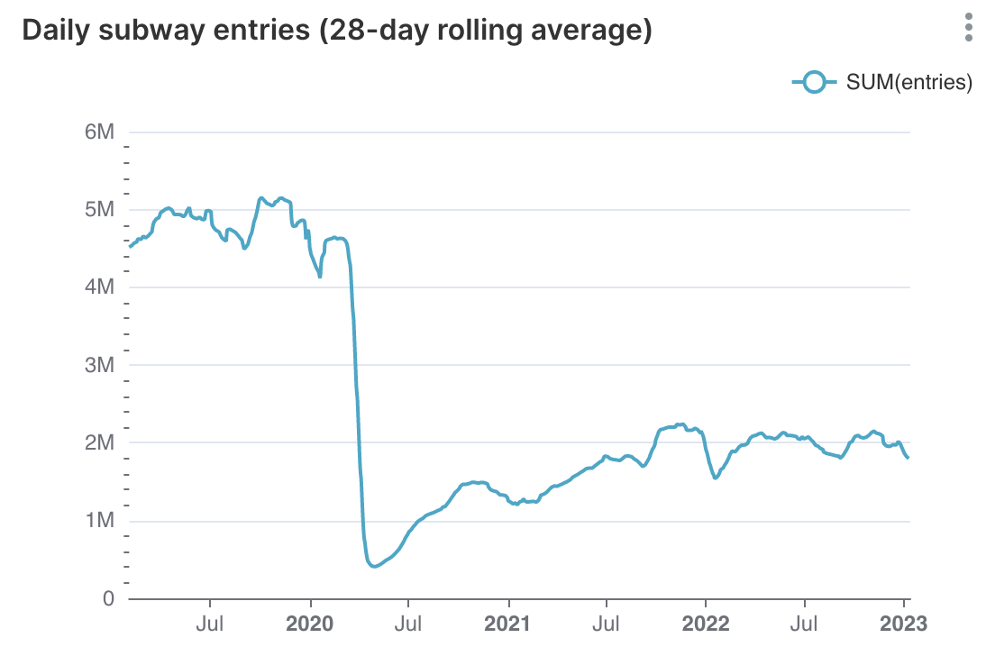
Numbers With Wings: A Modern Data Stack-In-A-Box
Not everything that counts can be counted, and not everything that can be counted counts. - Albert Einstein
There are three kinds of people: those who can count, and those who can’t. - Source unknown
-
Kant, Nietzsche, Elon Musk, SBF, wokeness, and the categorical imperative
I beseech you, in the bowels of Christ, think it possible you may be mistaken. - Oliver Cromwell
-
Time Series Analysis In Theory
- A regular time series is a function from integers to real numbers: \(y_t = f(t)\).
- Many useful time series can be specified using linear difference equations like \(y_t = k_1y_{t-1} + k_2y_{t-2} + \dots + k_ny_{t-n}\)
- This recurrence relation has a characteristic equation (and matrix representation), whose roots (or matrix eigenvalues) can be used to write closed-form solutions like \(y_t=ax^t\).
- Any time series combining exponential growth/decay and sinusoidal components can be modeled by a linear difference equation or its matrix representation.
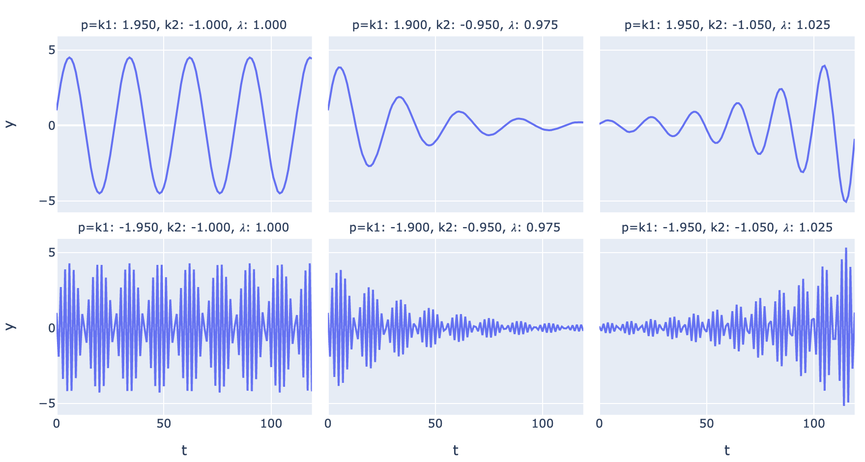
Fig. 1. Possible regimes for a 2nd-order linear difference equation with complex eigenvalues -
How I learned to stop worrying and love PCA: The optimal threshold for PCA dimensionality reduction
PCA is an essential data science tool which uses the SVD to break down the linear relationships in data. The Gavish-Donoho optimal truncation threshold provides a simple formula to select a good threshold for dimensionality reduction.
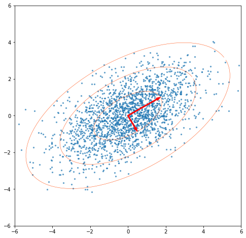
Fig. 1. A random 2D data set with singular vectors scaled by singular values -
Crypto systems, iron laws, and levels of resilience
Meditating on practical open distributed computing, how to build un-take-down-able apps like Web3 but without permissionless blockchains.
-
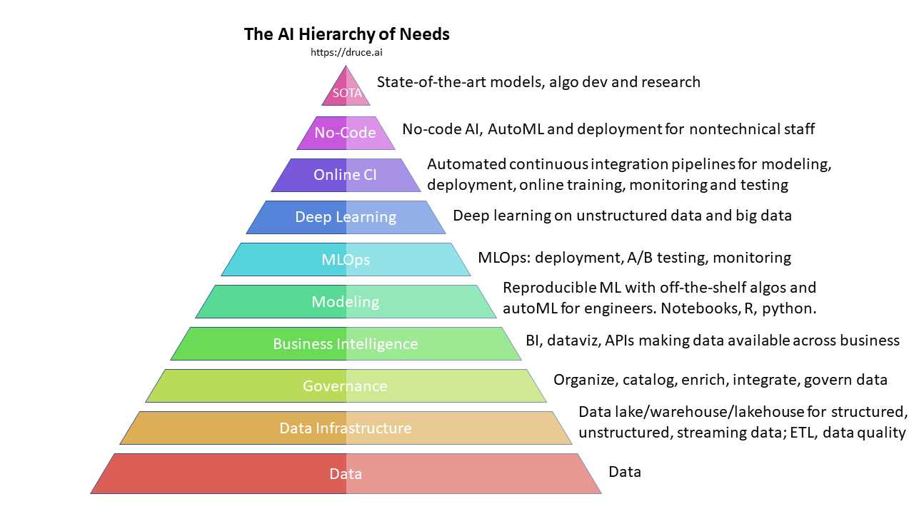
The AI Hierarchy of Needs
The perpetual challenge is building upper tiers before lower tiers are 100%, and strengthening lower tiers without breaking upper tiers.
-
Optimal Safe Withdrawal for Retirement Using Certainty-Equivalent Spending, Revisited
Revisiting Bengen’s “4% Rule” at various levels of risk aversion, and generalizing beyond a simple fixed-withdrawal, no-shortfall rule, to flexible rules at different levels of risk aversion.
-
What I would have written if I were Jack Dorsey
“Our decision to permanently suspend Donald Trump from the Twitter platform, may be a major inflection point in Twitter’s history. As CEO, I owe our users and employees a clear statement of why we took this action and how this decision evolved, i.e. not just some pablum about what a hard decision and potentially dangerous decision it was.”
-
Demystifying Portfolio Optimization with Python and CVXOPT
Do you want to do fast and easy portfolio optimization with Python? Then CVXOPT, and this post, are for you! Here’s a gentle intro to portfolio theory and some code to get you started.
-
Beyond Grid Search: Using Hyperopt, Optuna, and Ray Tune to hypercharge hyperparameter tuning for XGBoost and LightGBM
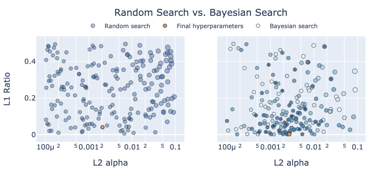
Bayesian optimization of machine learning model hyperparameters works faster and better than grid search. Here’s how we can speed up hyperparameter tuning using 1) Bayesian optimization with Hyperopt and Optuna, running on… 2) the Ray distributed machine learning framework, with a unified API to many hyperparameter search algos and early stopping schedulers, and… 3) a distributed cluster of cloud instances for even faster tuning.
-
Deploy a Microservice to AWS Elastic Container Service: The Harder Way and the Easier Way
A while back I made this Pizza service weekend project and I thought I could just press a button in AWS and deploy it in the cloud. It turned out to be… more complicated. With the latest version of Docker it’s getting easier. Here’s the harder (old) way and the easier (new) way. After some configuration, you can just say
docker compose upand your container is deployed. -
Cookie Cutter Machine Learning with Docker
A Docker configuration for machine learning
-
The Biggest Bluff: She Stoops To Conquer

I loved The Biggest Bluff: How I Learned to Pay Attention, Master Myself, and Win, by Maria Konnikova.
-
Deep Reinforcement Learning For Trading Applications (Alpha Architect)
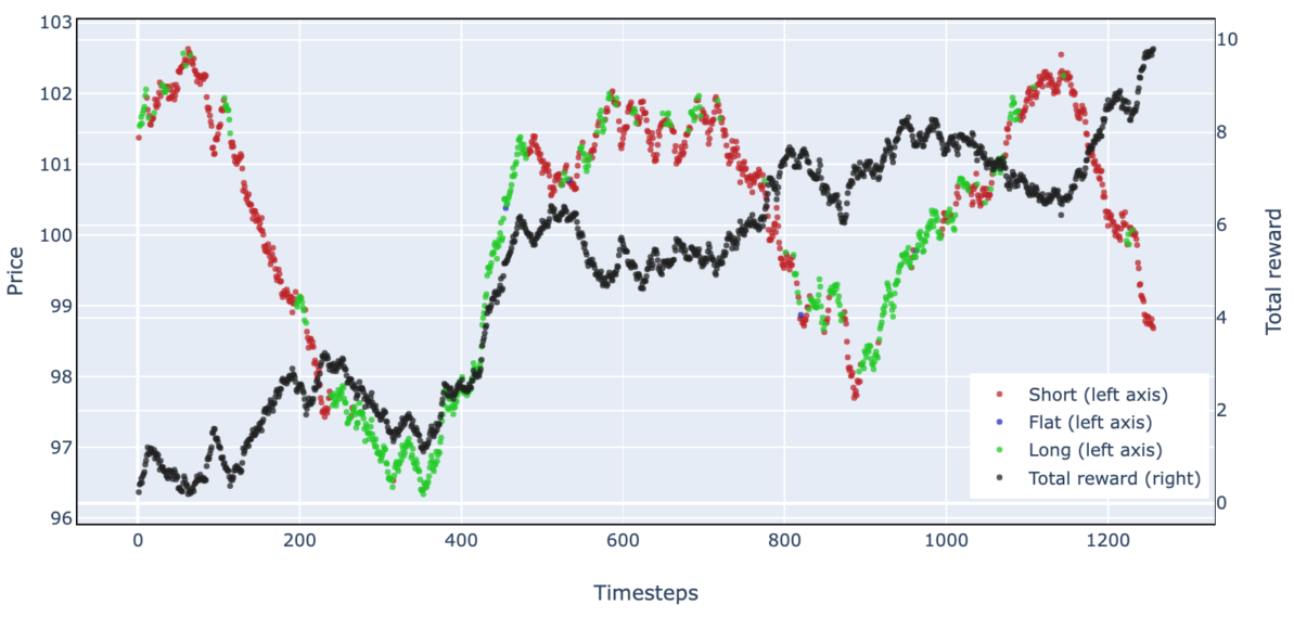
Reinforcement learning is a machine learning paradigm that can learn behavior to achieve maximum reward in complex dynamic environments, as simple as Tic-Tac-Toe, or as complex as Go, and options trading. In this post, we will try to explain what reinforcement learning is, share code to apply it, and references to learn more about it. First, we’ll learn a simple algorithm to play Tic-Tac-Toe, then learn to trade a non-random price series. Finally, we’ll talk about how reinforcement learning can master complex financial concepts like option pricing and optimal diversification.
-
Forecasting US Equity Market Returns with Machine Learning (Alpha Architect)
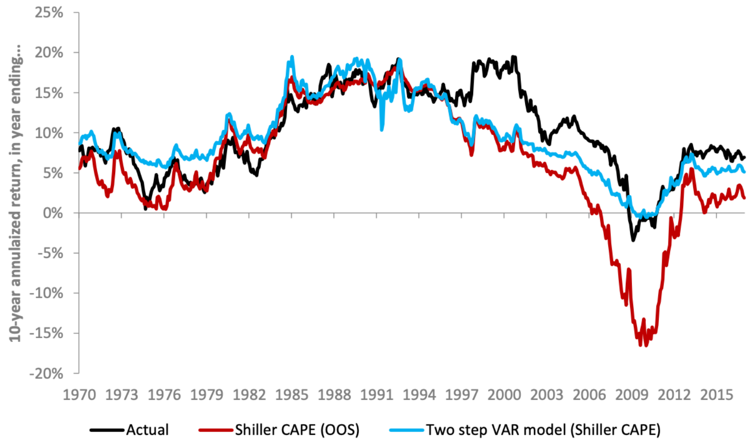
Shiller’s CAPE ratio is a popular and useful metric for measuring whether stock prices are overvalued or undervalued relative to earnings. Recently, Vanguard analysts Haifeng Wang, Harshdeep Singh Ahluwalia, Roger A. Aliaga-Díaz, and Joseph H. Davis have written a very interesting paper on forecasting equity returns using Shiller’s CAPE and machine learning: “The Best of Both Worlds: Forecasting US Equity Market Returns using a Hybrid Machine Learning – Time Series Approach“, which effectively applies machine learning to an import investing problem. Image source: Improving U.S. stock return forecasts: A “fair-value” CAPE approach, Joseph Davis, et al. (2017)
-
Understanding Classification Thresholds Using Isocurves
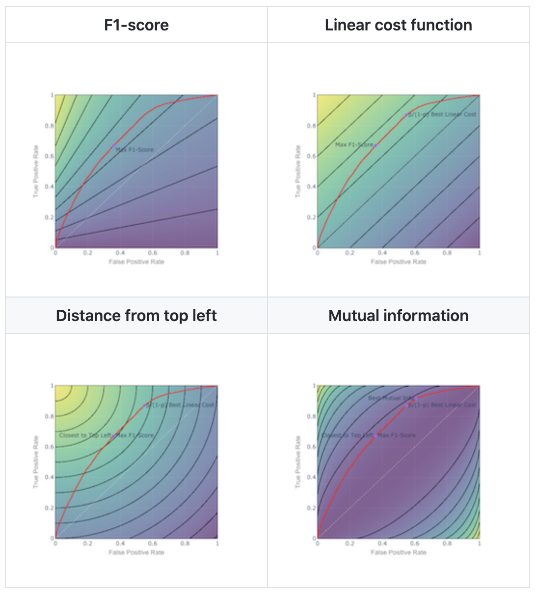
As a data scientist, you might say…“A blog post about thresholds? It’s not even a data science problem, it’s more of a business decision.” And you would not be wrong! Threshold selection lacks the appeal of say, generative adversarial networks.
-
Why Blockchain Is (Mostly) Useless
Strong State
Able to repress cryptoWeak State
Unable to repress cryptoHigh trust society
Low demand for cryptoUSA
Europe
Japan??? Island paradises ???
Polynesia?
Bhutan?Low trust society
High demand for cryptoChina
North KoreaVenezuela
SomaliaCryptocurrencies are useless. They’re only used by speculators looking for quick riches, people who don’t like government-backed currencies, and criminals who want a black-market way to exchange money. - Bruce Schneier
-
There ain't no such thing as a free option
I would not give a fig for the simplicity this side of complexity, but I would give my life for the simplicity on the other side of complexity. - Oliver Wendell Holmes
-
On the end of the StreetEYE experiment.
The StreetEYE news aggregator experiment came to an end on 3/31/2019. Many thanks for supporting StreetEYE over the years!
-
How I learned to stop worrying and love quantitative tightening
Many people are talking about ‘quantitative tightening’ and ‘balance sheet reduction’, and some people are blaming it for market volatility, discussed here, here, here. IMHO, blaming balance sheet reduction for market volatility is cargo cult mumbo jumbo.
-
The Top 100 People To Follow For Financial News On Twitter, January 2019
It’s been more than a year since we posted our last list of people to follow on Twitter for financial news. Time for an update!
-
Machine Learning Classification Methods and Factor Investing (Alpha Architect)
In this piece, we review machine learning methods for classification. Then we apply classification to the classic value/momentum factors (spoiler: the results are a bit too good).
-
Jupyter Notebook on an AWS instance
This is a tutorial on running Jupyter Notebook on an Amazon EC2 instance. It is based on a tutorial by Chris Albon, which did not work for me immediately (itself based on a tutorial by Piyush Agarwal). But I tweaked a few things and got it working.
-
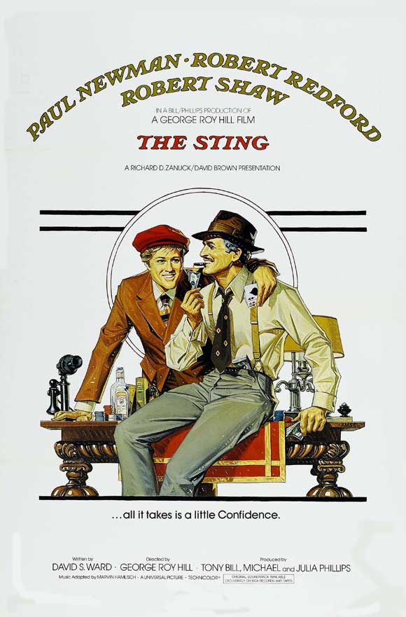
What I Learned From Watching The Sting And Reading David Maurer
 Wall Street never changes, the pockets change, the suckers change, the stocks change, but Wall Street never changes, because human nature never changes. _ Jesse Livermore
 -
The Most Shared Financial Blogs 2018
About once a year I’ll post the top Twitter accounts to follow. It’s a fun piece of social media analytics, and I’ll try to do it again later this year, after seeing if I can sidestep Twitter’s efforts to cut me off.
-
Machine Learning for Financial Market Prediction — Time Series Prediction With Sklearn and Keras (Alpha Architect)
We explore the paper “Dynamic Return Dependencies Across Industries: A Machine Learning Approach”, by David Rapach, Jack Strauss, Jun Tu and Guofu Zhou, and then try to improve the results with more sophisticated machine learning approaches.
-
Losing the meta-game
I suggest a new strategy, R2. Let the Wookiee win._ _ C3PO
-
Quantitative Fun With Fund Names
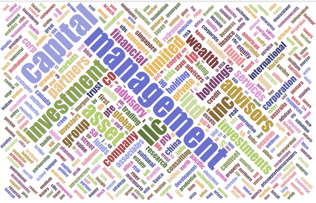 There are a number of hard problems in investing, for instance: 1) Finding alpha. 2) Finding clients and assets — especially if you can’t 1) consistently find alpha. 3) Finding an awesome name for your fund. The investing blogosphere is all over the first two. Now, for something completely different, we help you with the last one!
 -
The Bitcoin crash is coming
 Bitcoin inventor Satoshi Nakamura closely monitors the launch of Bitcoin futures (photo via @vexmark)
 -
Guns
 Here’s a Sunday rant on guns.
 -
Machine Learning for Investors: A Primer (Alpha Architect)
If you are out to describe the truth, leave elegance to the tailor. - Albert Einstein
-
A Google teachable moment, or the end of Western civilization?
 This anti-diversity manifesto has been making the rounds, with calls to avoid “socially engineering” diversity in response to “veiled left ideology”, to “de-moralize diversity”, to “de-emphasize empathy”, to “prioritize intention”, and to “be open about the science of human nature” which is claimed to confirm a lot of right-wing priors and stereotypes.
 -
UBI, health care, welfare economics and asshole economics
People sometimes ask me what I think about Universal Basic Income (UBI).
-
The Top 100 People To Follow To Discover Financial News On Twitter, May 2017
I posted earlier about some of the trends in the financial Twittersphere. It’s been a year since we posted our last list of people to follow on Twitter for financial news. Time for an update!
-
Rethinking the marketplace of ideas
I was recently listening to Fred Wilson and Howard Lindzon talk about, among others, news sources and curation, which is a topic dear to my heart. (Which I wrote about before here and here).
-
Come back Kelly Evans! We'll be good this time! I promise!
If we’d been born where they were born and taught what they were taught, we would believe what they believe. _ attributed to Abraham Lincoln. A digressive rant on the rot in the financial Twittersphere in the Trump era.
-
Some fun data-mining of StreetEYE headlines
Belated end-of-year roundup.
-
Is Silicon Valley Truly Libertarian? Is Politics Society's OS, Ripe For Disruption?
A hero is someone who understands the responsibility that comes with his freedom. _ Bob Dylan
-
Buyer’s markets, seller’s markets and the hedge fund hype cycle
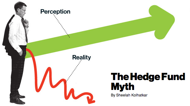 First come the innovators…Then come the imitators…And then come the idiots — Warren Buffett
 -
"Fake news", market designs, and the fascist/libertarian nexus
Arbitrary power is most easily established on the ruins of liberty abused to licentiousness. - George Washington.
-
Everyone lives in a bubble, and all models are overfitted
I beseech you, in the bowels of Christ, think it possible you may be mistaken. - Oliver Cromwell
-
Safe Retirement Spending Using Certainty Equivalent Values and TensorFlow
Certainty equivalent value is the concept of applying a discount to a stream of cash flows based on how variable or risky the stream is…like the inverse function of the risk premium.
-
The Game Theory of Assholes
The reasonable man adapts himself to the world; the unreasonable one persists in trying to adapt the world to himself. Therefore, all progress depends on the unreasonable man. - George Bernard Shaw
-
Pokémon economics, secular stagnation, and cognitive dissonance
There are these two young fish swimming along, and they come across an older fish swimming the other way, who nods at them and says, “Morning, boys, how’s the water?” And the two young fish swim on for a bit, and then eventually one of them looks over at the other and goes, “What the hell is water?” David Foster Wallace
-
A fun 3D visualization of the financial Twittersphere
Here’s a fun little update of that visualization of the financial Twittersphere I posted in May. This one is in 3D, you can zoom (with scroll wheel) and drag it around (with mouse, also see controls in top right).
-
Negative interest rates are an unnatural abomination
Mayor: What do you mean, “biblical”?
-
Hillary’s damn emails
The soldier who loses his rifle faces harsher punishment than the general who loses the war. — Anonymous soldier
-
The Top 100 People To Follow To Discover Financial News On Twitter, May 2016
It’s been a year since we posted our last list of people to follow on Twitter for financial news. Time for an update!
-
A possibly ill-conceived rant on race in America
There is no racial bigotry here. I do not look down on n******s, kikes, wops or greasers. Here, you are all equally worthless. _ Gunnery Sergeant Francis Hartman
-
What if everyone was a passive investor except Warren Buffett?
This is a slightly extended “director’s cut” of a post written for CFA Institute Enterprising Investor.
-
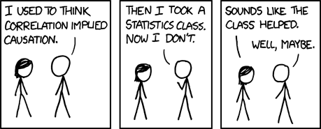
Narratives Are Powerful, But Check the Math
The first principle [of scientific inquiry] is that you must not fool yourself – and you are the easiest person to fool _ Richard Feynman
-
iPhone Backdoors for the FBI, a blockchain approach for transparent due process, and why it’s a bad idea
The national security complex is putting on the full court PR press for encryption back doors. See here and here. Basically this is about giving someone a TSA lock to your phone and promising to keep it really really safe unless a legit law enforcement request is received. Of course, legitimacy is in the eye of the beholder.
-
The most popular keywords and sites of 2015
Here’s a word cloud of StreetEYE headlines in 2015 (click to embiggen).
-
The End of the PC? On Intel’s Apple and ARM problems
 Tim Cook has been running around heralding the end of the PC. A self-serving assessment, but Intel and the PC ecosystem are going to struggle to maintain their traditional relevance. In this post, I will look at 1) the narrowing Intel/ARM performance gap, and 2) what the ‘end of the PC’ might look like.
 -
Is China’s sale of Treasurys ‘quantitative tightening’ for the US?
There’s this notion going around that since the Fed buying Treasurys was QE, therefore China selling Treasurys constitutes monetary tightening. Nope. The root cause of the disequilibrium and resulting capital flows is capital flight from China to the US.
-
The tontine: funny French name, brilliant idea
A hard problem in retirement planning is a safe spending rate, so you don’t outlive your money.
-
God help us
A rant on politics for a Labor Day weekend.
-
Smart Beta: Maybe Smart, But Definitely Not Beta
 A donut with no hole, is a danish. Ty Webb
 -
The Mathematics of Bluffing
A quick post about poker! That seemingly simple, deceptively complex game with a number of interesting parallels to investing. I just watched the MIT lectures on ‘Poker Theory and Analytics,’ an ‘Independent Activities Period’ mini-course, and for our mutual amusement, I worked through the math on bluffing, which is an interesting problem I had never done the full deep dive into. Here it is, including a Mathematica notebook.
-
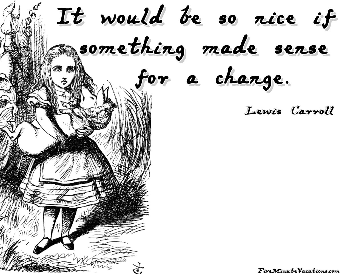
Through the Looking Glass
 Curiouser and curiouser! — Alice in Wonderland. Having written about Greece the last couple of weeks, why stop now?
 -
The Garbage Fire That is Greece
So, last week I said, Greece was getting booted out of the eurozone.
-
4 blinding glimpses of the obvious on Greece
More than any time in history mankind faces a crossroads. One path leads to despair and utter hopelessness, the other to total extinction. Let us pray that we have the wisdom to choose correctly. — Woody Allen
-
Why does everyone hate libertarians?
Rightful liberty is unobstructed action according to our will within limits drawn around us by the equal rights of others. Thomas Jefferson
-
Don’t feed the trolls
 There will always be those who mean to do us harm. To stop them, we risk awakening the same evil within ourselves. — James T. Kirk_
 -
Are food stamps Walmart subsidies, and should the minimum wage be $15?
There are a thousand hacking at the branches of evil to one that is striking at the root, and it may be that he who bestows the largest amount of time and money on the needy is doing the most by his mode of life to produce that misery which he strives in vain to relieve. – Henry David Thoreau
-
The Top 100 People To Follow On Twitter For Financial News
A couple of days ago I posted Mapping the Financial / Media Twittersphere, an illustration of the Twitter accounts that are most central for financial news.
-
Mapping the Financial / Media Twittersphere
The good folks at Captain Economics did a great post a couple of weeks back on ‘The Economics Twitosphere Top 100 Influential Users’.
-
Why Are There Recessions And Business Cycles?
 To everything, turn, turn, turn.
There is a season, turn, turn, turn.
And a time to every purpose under heaven.
The Byrds, by way of Ecclesiastes
To everything, turn, turn, turn.
There is a season, turn, turn, turn.
And a time to every purpose under heaven.
The Byrds, by way of Ecclesiastes -
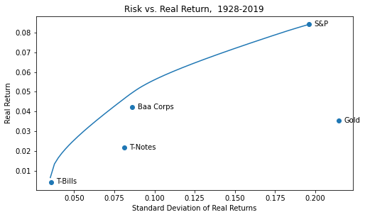
Gold as Part of a Long-Run Asset Allocation (update)
You have to choose between trusting to the natural stability of gold and the natural stability of the honesty and intelligence of the members of the government. And, with due respect to these gentlemen, I advise you, as long as the capitalist system lasts, to vote for gold. - George Bernard Shaw
-
Good risks and bad risks
 Matthias Steiner, Beijing 2008. Pain is weakness leaving the body, and/or your central nervous system telling you you’re about to die. - source unknown
 -
‘Net neutrality’, Netflix vs. the cable monopoly, and the Internet profits tax
Really, the way to understand ‘net neutrality’ is it’s all about Netflix. The cable companies are outraged and scared to death about Netflix. If you’ve tried a Roku Internet TV appliance (or Apple TV, or Google Chromecast, or Amazon Fire TV), it’s a 10x user experience improvement on a cable box. For less money.
-
Andreessen v. Summers: Can you have robots, hoverboards, and secular stagnation?
Diane Coyle says you can have either robots, or secular stagnation, but not both. In a somewhat confused tweetstorm, Marc Andreessen says secular stagnation is BS. Larry Summers, who is one of the guys behind the secular stagnation hypothesis, responds. But then, confusingly, is reported to agree with Coyle.
-
Game theory, Bill Belichick, Neville Chamberlain
There are some people that will be deterred by the fact that we have nuclear weapons… But those people are the folks we can deal with anyway. — General Charles Horner. Sometimes it pays to be irrational, to do the unexpected like pass on 2nd and 1, to catch the defense by surprise. If one believes the evil genius of Belichick, he got inside Carroll’s OODA loop, he psyched Carroll into calling it and anticipated him.
-
A Greece reading list (Or why the euro is doomed)
Time converts the improbable to the inevitable – Stephen Jay Gould. [TL;DR 50% odds Greece leaves euro this year. Odds eurozone breaks up eventually: ~100%]
-
PCs Were the Triumph of the Nerds; iPhone is the Revenge of the Cool Kids
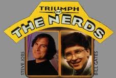 *Apple reported a blowout iPhone 6 launch quarter. In fact, reportedly the largest quarterly profit ever reported by a public company. I had a feeling they would blow away expectations, the iPhone 6 looks and feels great, it’s a must-have upgrade. *
 -
The Dark Web Stack, Or How To Eff Up The Net
 An interesting dive into “Deep Web Marketplaces” by the folks at avc.com and USV. You have a choice of trusting the natural stability of gold or the honesty and intelligence of members of the government, and with all due respect to these gentleman, I advise you as long as the capitalist system lasts, vote for gold. – George Bernard Shaw
 -
UberFail - a few thoughts on Uber
To lose one parent, Mr. Worthing, may be regarded as a misfortune; to lose both looks like carelessness. _ Oscar Wilde, The Importance of Being Earnest
-
A Piketty counterargument: Is r > g a reasonable assumption?
A thought experiment: If you could buy an asset that returned the GDP growth rate, would you, should you do it?
-
Risk: Visualizing Diversification With Risk Triangles
 In this post we’re going to look at a simple way to visualize the power of diversification, and what correlation really tells us.
 -
Risk: Why is volatility used to measure risk?
Volatility is a proxy for how risky Mr. Market thinks an asset is.
-
Retirement plans that maximize certainty-equivalent spending (conclusion)
In part 1 and part 2, we developed a framework for evaluating and identifying a good plan for retirement spending and asset allocation.
-
Retirement plans that maximize certainty-equivalent spending, part 2
Last time we solved the problem of the perfect retirement spending plan, assuming a fixed known real return, and a CRRA utility function.
-
Optimal certainty-equivalent spending retirements with DataNitro
*Let’s see if we can come up with an ideal spending plan for a retirement, if you have a guaranteed annual return, for different levels of risk aversion. *
-
Bitcoin is the Linux of payments. And its killer apps will be for US dollars.
 I was scanning the news the other day, and someone on Hacker News mentioned that half the items above the fold on StreetEYE were about Bitcoin. And I said to myself, I haven’t seen the neckbeards this excited since the early days of Linux. And it hit me, Bitcoin is the new Linux.
 -
Why Bitcoin is here to stay
 . In 2011 I blogged about why Bitcoin is a Ponzi scheme doomed to fail.
 -
Amazon is making money
 Profits, like sausages… are esteemed most by those who know least about what goes into them. Alvin Toffler
 -
The StreetEYE manifesto
") “Being good…is not good enough! Everyone must be connected to our strategy, or we will find you, and weed you out! Information arbitrage is our business. If you don’t know what an information curve is, then find out! Position yourself in an information curve. Dominate the curve! Nick Leeson, who most of you know and all of you have heard of, runs our operation in Singapore, which l want all of you to try to emulate.” — Ron Baker, in Rogue Trader (1999)
“Being good…is not good enough! Everyone must be connected to our strategy, or we will find you, and weed you out! Information arbitrage is our business. If you don’t know what an information curve is, then find out! Position yourself in an information curve. Dominate the curve! Nick Leeson, who most of you know and all of you have heard of, runs our operation in Singapore, which l want all of you to try to emulate.” — Ron Baker, in Rogue Trader (1999) -
Obama goes all-in on Inspector Clouseau for the Fed
 So, the Obama Administration is ‘all-in’ on Summers, despite nearly everyone who hasn’t worked for him (and a number who have) thinking he’s not the best candidate.
 -
Risk arbitrage _ Investing and poker
When I was young people called me a gambler. As the scale of my operations grew, I became known as a speculator. Now I am called a banker. But I have been doing the same thing all the time. - Ernest Cassel
To win, you must understand the game, you must understand the players, and above all you must understand yourself. - Source unknown
-
“Cat Food” Revisited: Final Thoughts - Part 4
Here is the long-awaited conclusion to the wonky 4-part discussion of safe retirement spending. We went pretty far down the rabbit hole, and I think the conclusions are useful.
-
‘Cat Food’ revisited – testing dynamic spending rules – Part 3
In the last part of our look at dynamic rules for spending in retirement, we discussed how changing the allocation between stocks and bonds affects the maximum sustainable spending rate. We can summarize this relationship by plotting the highest feasible initial spending rate for any acceptable shortfall level.1
-
‘Cat Food’ revisited – testing dynamic spending rules – Part 2
The last post discussed a framework for evaluating simple dynamic spending rules.
-
‘Cat Food’ revisited: testing dynamic spending rules - Part 1
How much can you safely spend out of a portfolio in retirement? Spend conservatively and you may be unnecessarily curbing the lifestyle and aspirations of you and your loved ones. Overspend and risk a shortfall and painful adjustment - in the extreme, the (hopefully apocryphal) “cat food” diet.
-
What’s the worst that could happen?
It’s not whether you get knocked down, it’s whether you get up. Vince Lombardi
-
‘Big Data’
If ‘The Graduate’ were made today, Benjamin Braddock might hear a well-meaning uncle stage-whisper ‘Big Data’ instead of ‘Plastics.’ (Runners-up: ‘The Cloud’, ‘Social Discovery’, ‘Gamification’, the list goes on.) ‘Big data’ is a buzzword that people throw around a lot. What does it mean? Large data sets are not new. The IRS, the Census, Walmart, money center banks have always had big data sets. What’s changed?
-
What I Learned
I didn’t really post as much as I would have liked this year.
-
Social capital, or the lost art of not taking a dump in the community pool
Everybody talkin’ to their pockets / Everybody wants a box of chocolates / And a long-stemmed rose - Leonard Cohen
-
Broken Windows
 So, some people are talking about Hurricane Sandy putting people back to work, and others are pointing out that this is the ‘broken windows fallacy.’ True, a massive superstorm is usually not a good thing. Nevertheless, three quick points.
 -
The Paul Ryan plan
The Paul Ryan plan ‘Promotes saving by eliminating taxes on interest, capital gains, and dividends; also eliminates the death tax.’
-
A Target2 Thought Experiment
There has been a lot of controversy about this process, and the notion that Germany will get stuck with massive losses if, following massive capital flight now in progress to Germany, the peripheral countries leave the euro.
-
Domino on the edge
“The crisis takes a much longer time coming than you think and then it happens much faster than you would have thought.” Rudiger Dornbusch.
-
Startup Growth v. Revenue
Nick Bilton points to the lack of revenue at startups as signs of a bubble.
-
How to Create the Ultimate Linkfest
At Linkfest.com, we love linkfests so much we named our website after them. When a knowledgeable professional is dedicated enough to get up at an ungodly hour to make an up-to-the-minute reading list for us, that just shows true love for the craft of investing, the game, and the readers. It just makes us warm and fuzzy.
-
The Money Illusion
") Irving Fisher is mostly remembered, a bit unfortunately, for writing that stock prices were at a permanently high plateau…right before the Great Crash of 1929. He also invented the Rolodex, pioneered early economic statistics-gathering, wrote of the Fisher money equation PY=MV and the Fisher debt-deflation cycle. (See Sylvia Nasar’s Grand Pursuit - interesting but wouldn’t consider it must-read.)
Irving Fisher is mostly remembered, a bit unfortunately, for writing that stock prices were at a permanently high plateau…right before the Great Crash of 1929. He also invented the Rolodex, pioneered early economic statistics-gathering, wrote of the Fisher money equation PY=MV and the Fisher debt-deflation cycle. (See Sylvia Nasar’s Grand Pursuit - interesting but wouldn’t consider it must-read.) -
The New Information Diet: Web and Social Media Best Practices For Investors
The History of every major Galactic Civilization tends to pass through three distinct and recognizable phases, those of Survival, Inquiry and Sophistication, otherwise known as the How, Why, and Where phases. For instance, the first phase is characterized by the question ‘How can we eat?’ the second by the question ‘Why do we eat?’ and the third by the question ‘Where shall we have lunch?” Douglas Adams
-
Steve Jobs, by Walter Isaacson
Finally got around to reading the Steve Jobs bio by Walter Isaacson. It’s must read for anyone involved in the tech business. Some slightly less charitable takes: John Gruber is all I Am Disappoint there aren’t more insights into the products and strategy. Self-described underemployed writer Maureen Tkacik notes that Jobs was a Machiavellian liar, exploiter, and control freak.
-
Buffett, Stocks, Bonds, Gold
Warren Buffett contributed a Fortune article with his customary paean to the virtues of stocks over the long term. There is some worthy discussion from John Hempton and the pseudonymous Kid Dynamite.
-
Is Facebook Worth $100B?
Since everyone else is playing the Facebook valuation parlor game, here is a stab at it.
-
Are long term asset class relationships stable?
Last week, we looked at gold as part of a long-term asset allocation. I was curious about how stable those relationships would be over time, so I ran the same plots, starting from different inflection points.
-
Portfolio Optimization and Efficient Frontiers in R
If you want to frustrate someone for a day, give them a program. If you want to frustrate them for a lifetime, teach them how to program.
-
Gold as Part of a Long-Run Asset Allocation
What does an efficient long-run portfolio look like for major US asset classes, and where does gold fit in?
-
Over-The-Top Speculations
Thinking about cord-cutting and over-the-top video like Netflix
-
2012: Toilet bowl or takeoff?
Some drive-by thoughts on Europe:
-
Once Again, Britain stands alone
Two differing views on UK and the EC.

-
Unstoppable Forces vs. Immovable Objects
") Europe is heading into yet another moment of truth this week, with a Merkozy summit and a new plan, an ECB meeting and likely interest rate cut, and a full EU summit starting Friday.
Europe is heading into yet another moment of truth this week, with a Merkozy summit and a new plan, an ECB meeting and likely interest rate cut, and a full EU summit starting Friday. -
Why only millionaires should play Powerball
 ROCKY HILL, Conn. — Three asset managers from Connecticut’s affluent New York suburbs claimed a $254 million Powerball jackpot on Monday off a $1 ticket.
 -
Margin Call - A Big Sell Out
 Watched Margin Call last night on iTunes and woke up cranky. Here is a short list of things that it gets wrong about Wall Street.
 -
Occupying Ourselves
 Never doubt that a small group of thoughtful, committed citizens can change the world; indeed it’s the only thing that ever has. - Margaret Mead
 -
Steve Jobs, 1955-2011
Steve Jobs was to tech like John Lennon was to music _ changed the game, launched a new era, had vision and integrity, was an inspiration to people.
-
Apocalypse Now?
 Larry Summers: Daniel Ellsberg drew out the lesson regarding the Vietnam War…Policymakers acted without illusion. At every juncture they made the minimum commitments necessary to avoid imminent disaster — offering optimistic rhetoric but never taking steps that even they believed offered the prospect of decisive victory. They were tragically caught in a kind of no man’s land — unable to reverse a course to which they had committed so much but also unable to generate the political will to take forward steps that gave any realistic prospect of success.
 -
Deleveraging: A Parable
It is a slow day in a small Irish town. The rain is misting and the streets are deserted. Times are tough, everybody is in debt, and having a hard time making ends meet, let alone climbing out of debt.
-
The Efficient Atmospheres Hypothesis
 A good analogy Of hurricanes and economic equilibrium.
 -
Random Tech Comments
Wild and woolly couple of weeks in tech world ‘out with the old, in with the new.’
-
Overhyped Economic Hurricane?
With the S&P down 13% since July 7, and the 10-year rate down a point to barely over 2%, markets are discounting the double dip. They might be doing a great job of early warning, sensitive to faint aromas in complex crosscurrents of data. Or they might be wrong.
-
‘Cat Food’ In An Age of Diminished Expectations
Tucked away in the neglected items in the ‘Tools’ menu above, you might have noticed the metaphorical ‘Cat Food Calculator’.
-
Lucky Duckies and Red Herrings
There’s a disingenuous meme being perpetuated by the grossly misinformed and cynical, that 50% of Americans get government benefits, but pay no taxes (the ‘lucky duckies‘, here and there and everywhere).
-
State of Play
We have been going through the stages of coming to terms with GOP berzerkers. 1. Denial: “They’re just posturing.” 2. Astonishment: “Wow, some of them are dumb enough to believe their own BS.” 3. Facepalm: “I can’t believe they’re actually going to do this.”
-
Fannie, Freddie, And The Causes Of The Financial Crisis
Once again, people are debating here and here and here whether the GSEs like Fannie Mae and Freddie Mac caused the financial crisis.
-
The debt limit and the bond market
Sometimes the first duty of intelligent men is the restatement of the obvious. - George Orwell
-
ETFs: Get Off My Lawn!
The greater the institution, the greater the chances of abuse. - Mohandas K. Gandhi
-
The Great Bitcoin Robbery
Bitcoin is a fascinating experiment: digital currency that doesn’t depend on a central authority.
-
100 traders, 100 boxes, part deux
A math/probability problem I think is awesome and counterintuitive, and may be instructive about financial markets: A hedge fund manager puts 100 traders in a room and instructs them: “On the trading desk, there are 100 boxes. Each box has one of your names. You can go [one at a time] onto the trading desk and open any 50 boxes you choose, to try to find your name. If every one of the 100 traders in this room finds his or her name, you will each get a $1,000,000 bonus. If anyone fails, I will crush all your $100,000 BMWs to create my modern art masterpiece. You can devise a strategy before anyone leaves the room, but once a trader has opened the boxes, you must leave the trading desk exactly as it was before you entered and cannot communicate with anyone else.”
-
We make our tools, and then our tools make us
 You didn’t change the game, the game changed you. Niko Bellic, Grand Theft Auto IV
 -
The bottom is always at least 10% below your worst case expectation
 ‘Black swan’ is a term which is overused and under-understood.
 -
What is money?
 *As far as the laws of mathematics refer to reality, they are not certain, as far as they are certain, they do not refer to reality. - Albert Einstein
 -
6 Reasons Why There Will Be No Chinese Jasmine Revolution
 The Chinese government has taken insecurity and paranoia up a notch in the wake of the Jasmine uprisings in the Arab world. They have ‘disappeared’ dissident artist Ai Weiwei and cracked down hard on human rights activists, meddlesome lawyers, and dissidents.
 -
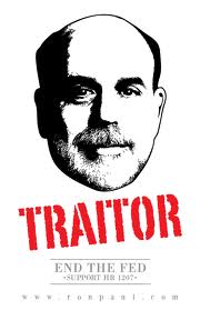
Questions for Gentle Ben
 A question for Ben Bernanke at today’s press conference:
 -
Can the US default on its debt?
*The S&P rating downgrade was deservedly greeted as a big joke. *
-
From the unthinkable to the inevitable: why the Euro is doomed
 The brilliant, provocative, and slightly mad GMU economist and blogger Tyler Cowen wrote his New York Times column about why the Euro zone is headed for breakup.
 -
Why I am not a libertarian
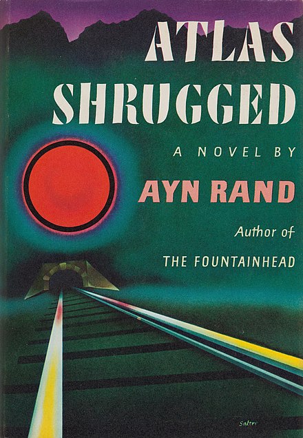 </a> I have been reading the poor reviews of Atlas Shrugged. I feel almost disappointed that it is by collective consensus a steaming turd. I would welcome a thoughtful movie about an interesting thought experiment, and I think the country could use a rare substantive debate about the size and role of government.
 -
‘Bretton Woods 2’
A lot of cool videos from INET’s Bretton Woods conference last week. Kind of like TED talks for econ supergeeks.
-
Why I am not a true gold bug, and the gold standard isn’t coming back
Let me say at the outset that I am bullish on gold in the long run. US demographics, politics, debt levels, harder-to-extract energy, peaking of globalization’s labor supply shock: all these point to inflation in the long run. And central bankers have not exactly covered themselves in glory lately. That being said, going back on the gold standard makes exactly as much sense as going back to horses and buggies. Here’s why.
-
Tech Trends
A few technology megatrends:
-
Red Capitalism, Potemkin Finance: Behind Facade Of Modern Buildings, Institutions, State Directs Dysfunctional Markets
China’s remarkable growth continues _ China has apparently now passed the US in industrial production, with the world GDP title in its sights (see previous post).
-
China’s economy: future world domination, or paper tiger?
China’s surge from basket case to the world’s factory is simply breathtaking. But the powerful rise has outpaced institutions that Westerners see as prerequisites to capitalism.
-
Why did the Soviet Union collapse?
A few years old, but new to me: an interesting perspective from Yegor Gaidar, reformist economist of the post-Gorbachev era.
-
China: society and politics, and what next?
In the post-war period period (possibly throughout the dynasties), truth has been relative in China, while power has been absolute.
-
China: A history primer
 I spent March in Asia and trying to figure out China. Here is a quick summary mixed with a few conclusions and speculations.


")


")


